Deep dive into telemetry, aerodynamics, and race strategy using Python, FastF1, and advanced analytics
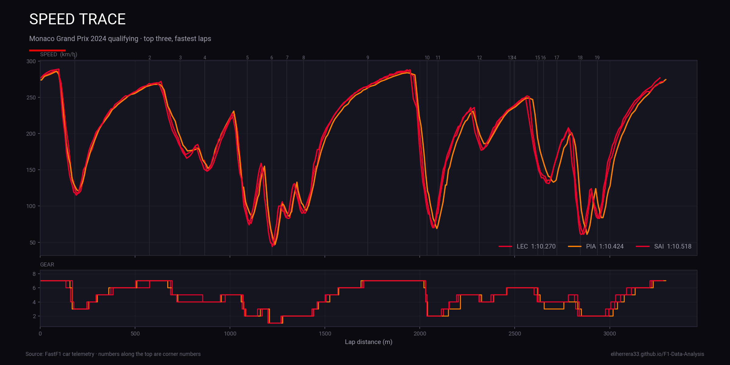
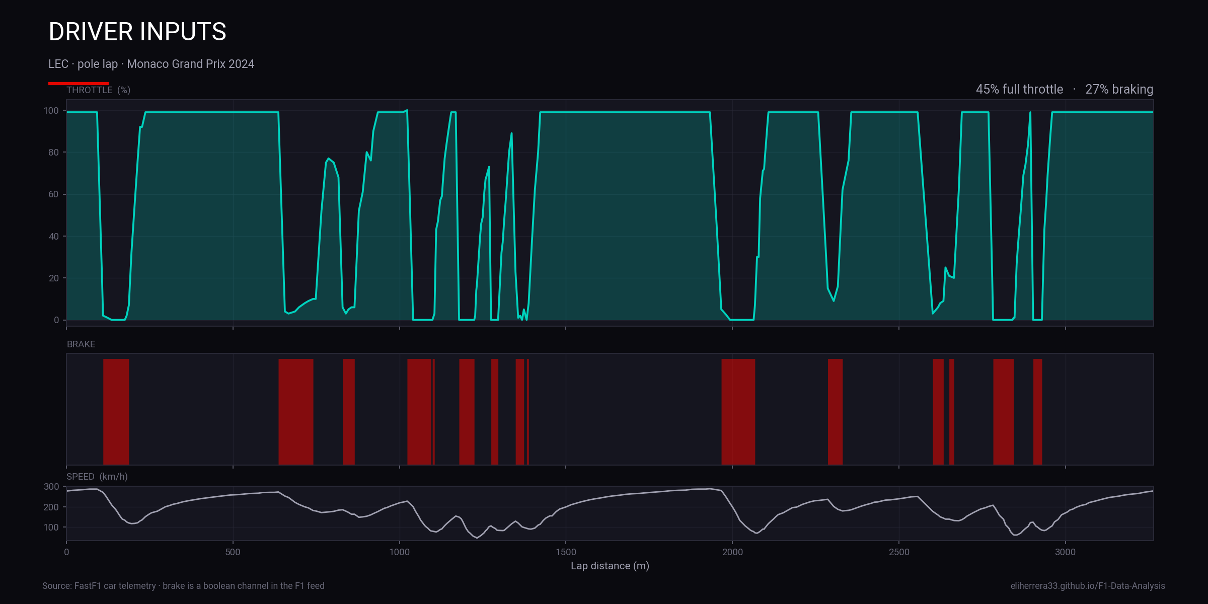
Real-time car data analysis including speed traces, throttle/brake application, and driver comparison
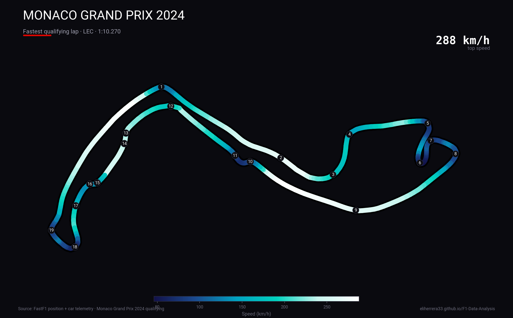
GPS-based track visualization with speed-colored trajectory showing where drivers gain and lose time
Lap-by-lap speed comparison revealing braking points and acceleration zones
Driver input analysis showing pedal application patterns and driving style
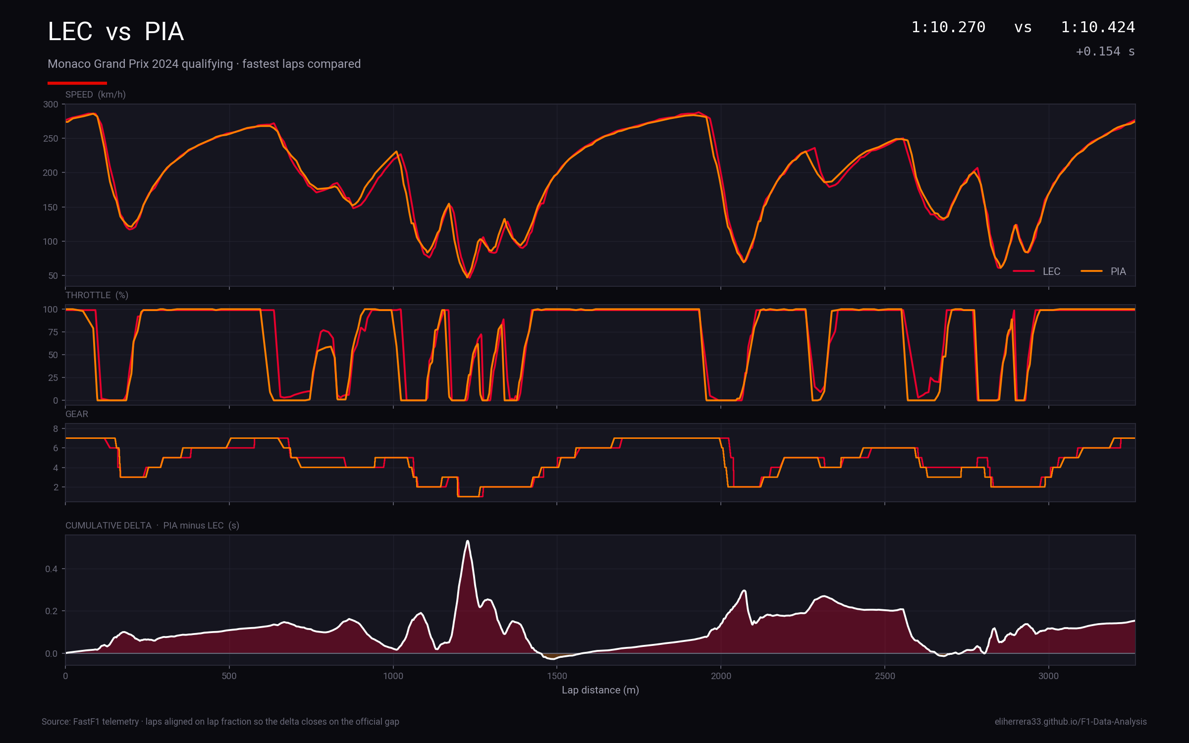
Head-to-head analysis of driver performance across all telemetry channels
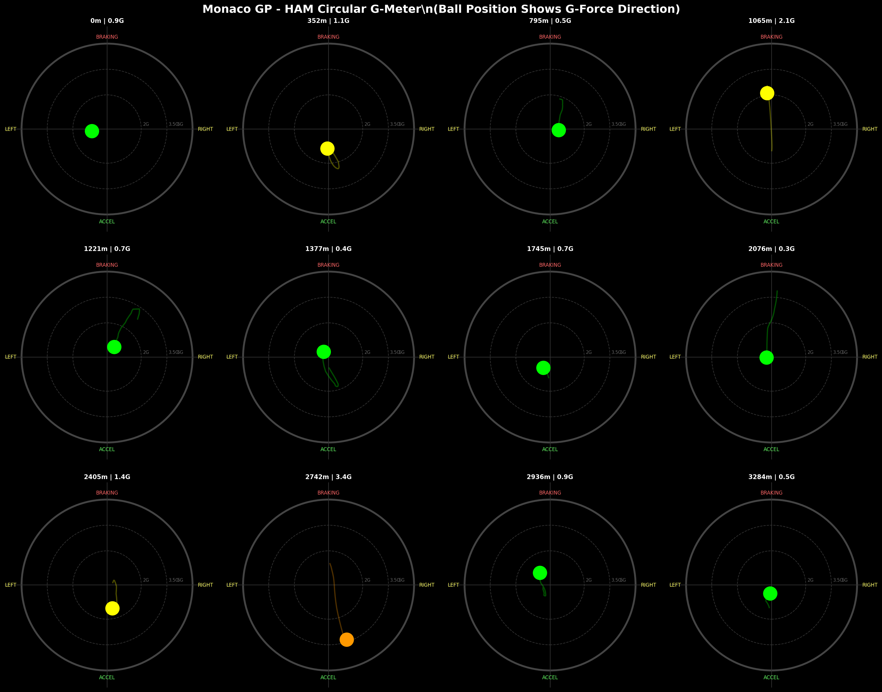
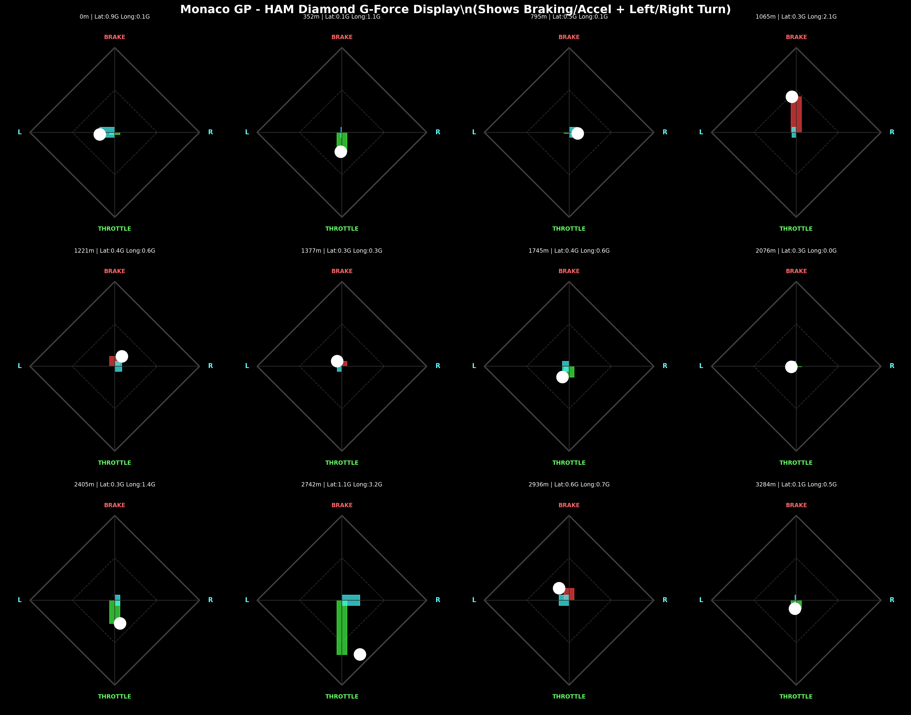
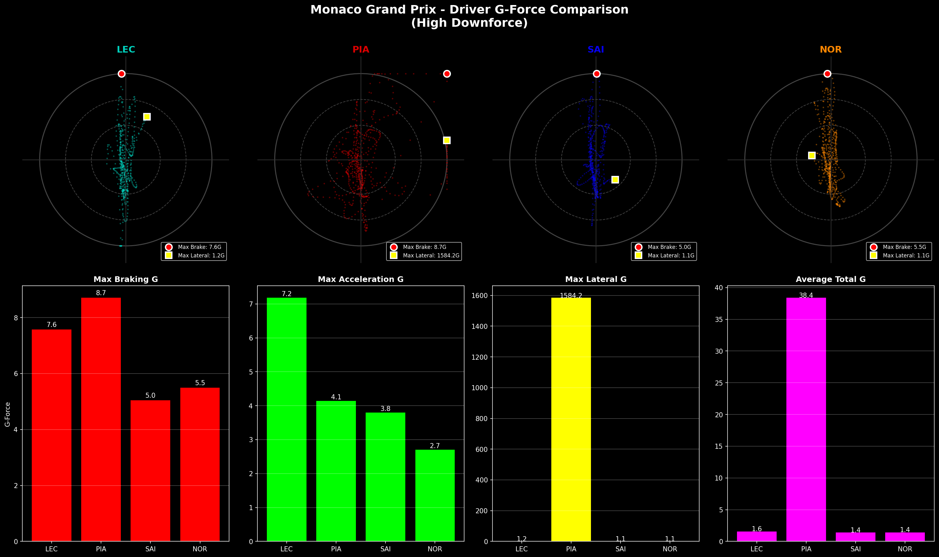
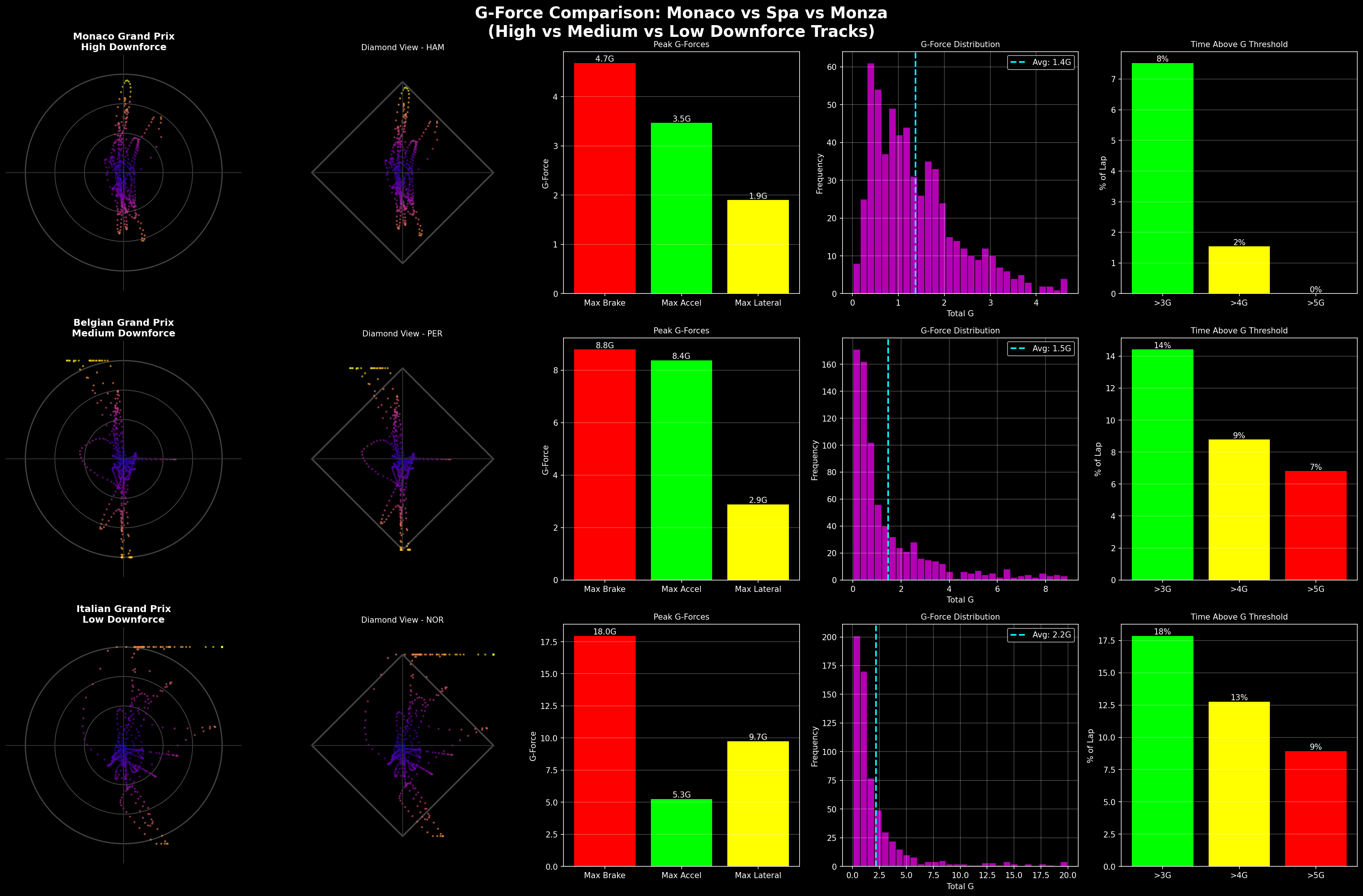
Calculate and visualize the extreme forces drivers experience - up to 6G in corners and under braking
Diamond Gauge
Driver Comparison
Track Comparison
Longitudinal deceleration calculated from speed derivative
a = Ξv / Ξt β G = a / 9.81
Cornering force from centripetal acceleration
a = vΒ² Γ ΞΊ β G = a / 9.81
Combined force magnitude on driver
G_total = β(G_longΒ² + G_latΒ²)
A live aerodynamic model you can drive. Change the setup and watch the flow field, the load split and the lap-time consequences move together.
The numbers come from the PERRINN 2017 open-source F1 CFD dataset
(windtunnel_data/perrinn_cfd_data.csv): sCz = 3.25 m²
and sCx = 1.16 m² at 40 mm front / 50 mm rear ride
height. Those coefficients already include the reference area, so force is
½ ρ v² sC — no second multiplication by frontal
area. Setup changes scale each component: wing load moves roughly linearly with angle while its
induced drag grows with the square, and the floor follows a ground-effect curve that peaks near
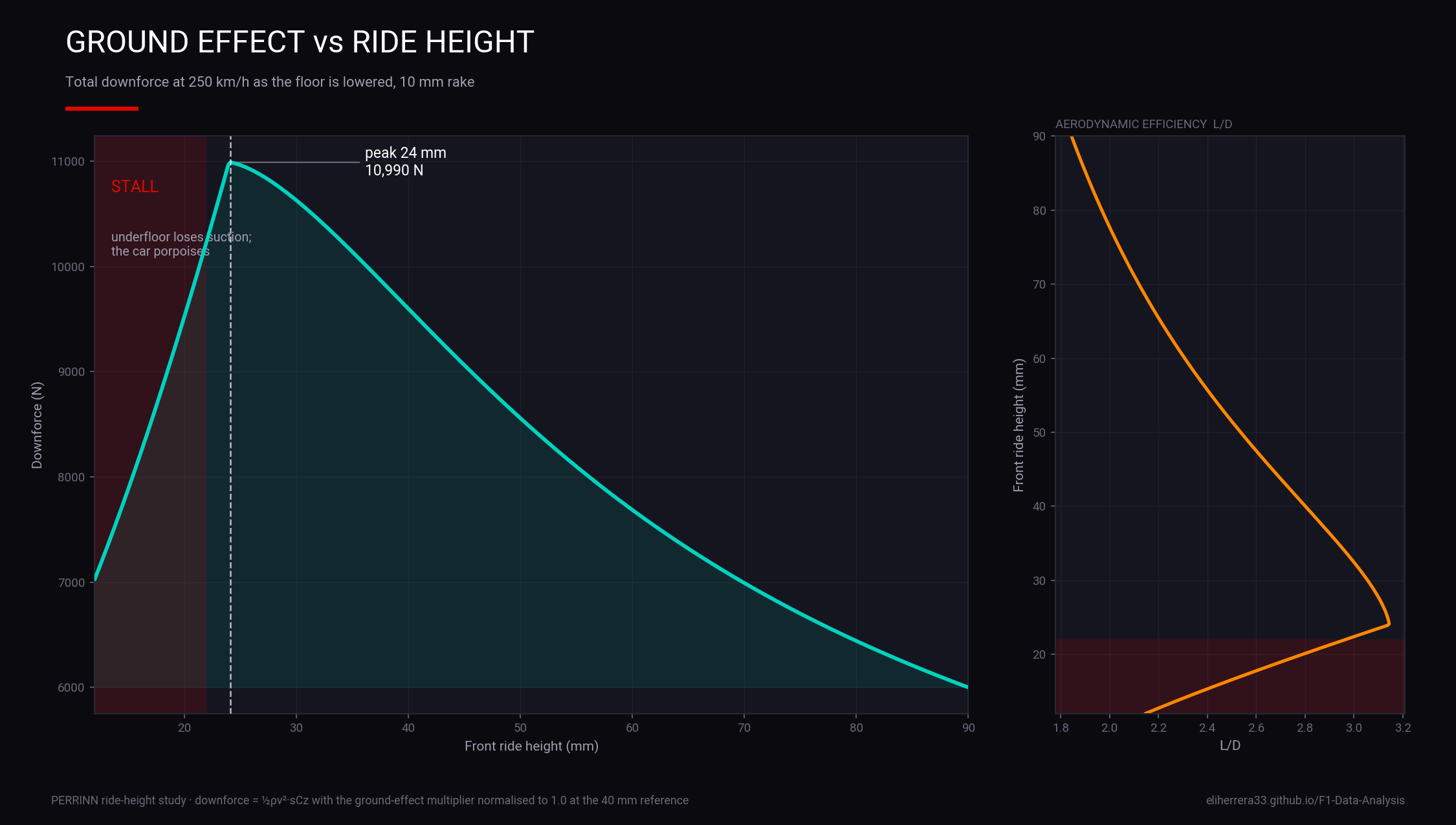
24 mm and collapses below it, which is the porpoising cliff the grid rediscovered in 2022.
The picture is a 2D potential-flow approximation: doublets give the body its
thickness, Rankine vortices carry the circulation, and every element is mirrored about the ground
plane so y = 0 stays a streamline. Circulation is divided between the front wing,
floor, diffuser and rear wing using the same split as the force model, so the flow and the readouts
always agree. Pressure colouring is Bernoulli:
Cp = 1 − (V/V∞)².
Streamline magnitudes are scaled for legibility — treat the flow as qualitative and the forces
as quantitative.
Run a lap is a quasi-steady lap-time model over the real pole lap's centreline: grip-limited speed at every point from the downforce your setup produces, a forward pass limited by the friction circle and by power against drag, and a backward pass for braking. Track curvature comes from the FastF1 position channel, smoothed with a Savitzky–Golay fit; DRS zones come from the pole lap's DRS channel where it exists and from the two longest full-throttle straights where it does not. Tyre grip and power were fitted so the fastest setup the model can find lands on the real pole time at all three circuits — the residuals are in the exported data. It is a first-order model: it has no tyre temperature, no wind, no kerbs and no driver.
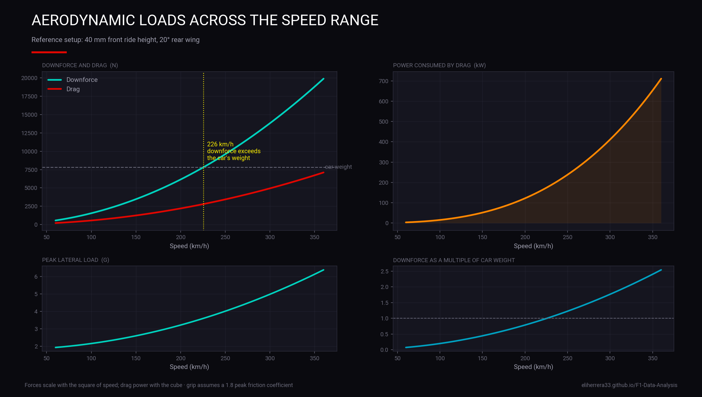
Grip assumes a peak slick friction coefficient of 1.8 on the combined weight and downforce; Vmax solves drag power against roughly 470 kW at the wheels, calibrated so a Monza DRS setup tops out around 355 km/h. Both are first-order estimates, not a lap simulation.
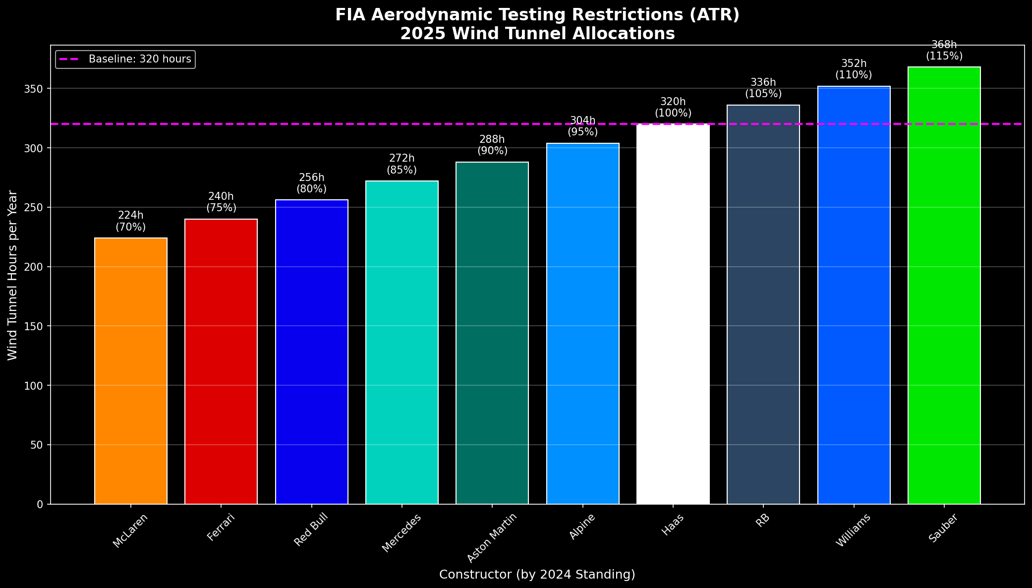
Formula 1 caps aerodynamic development on a sliding scale: finish higher, get less wind tunnel time. Pick a position to see what each team is allowed.
The allocation runs from 70% of the baseline for the constructors' champion to 115% for tenth. It applies to both wind tunnel runs and CFD items, and it resets against the standings twice a season — so a mid-year climb up the table costs a team development time for the run-in.
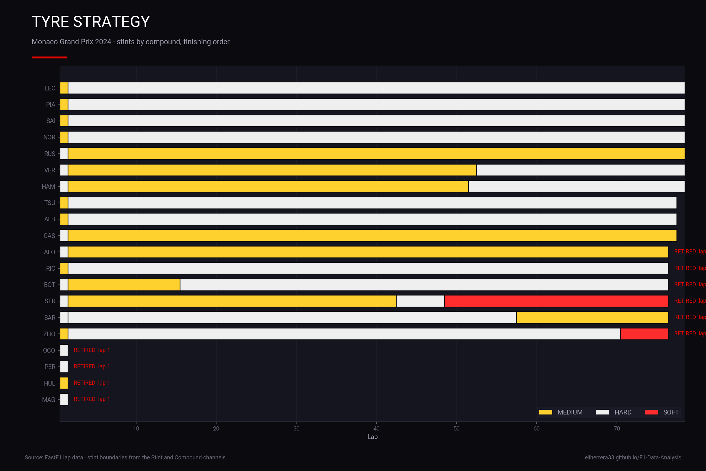
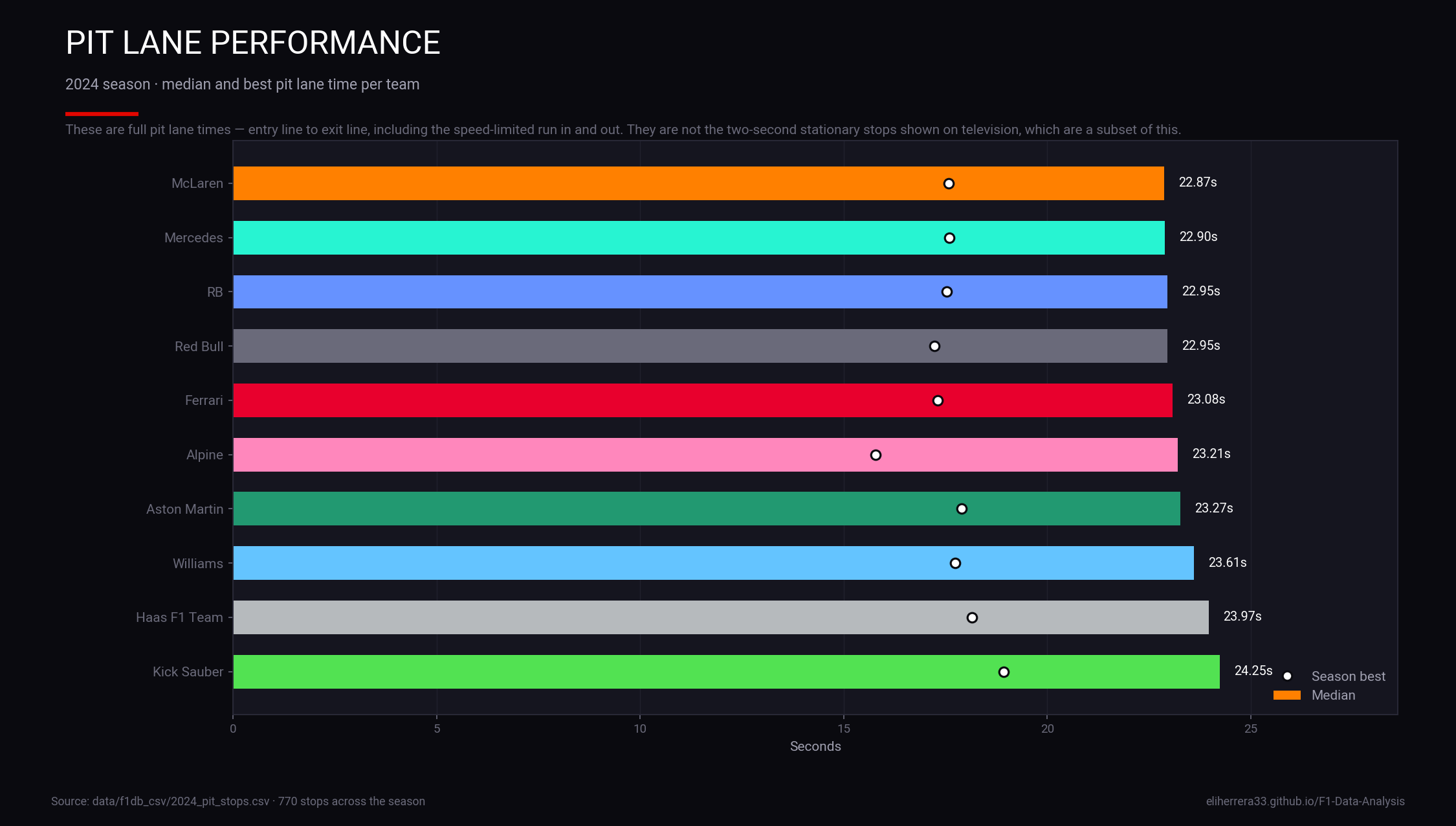
Tire compound analysis, pit stop optimization, and degradation modeling
Compound usage per driver visualized across race distance
Team pit stop times analysis and comparison
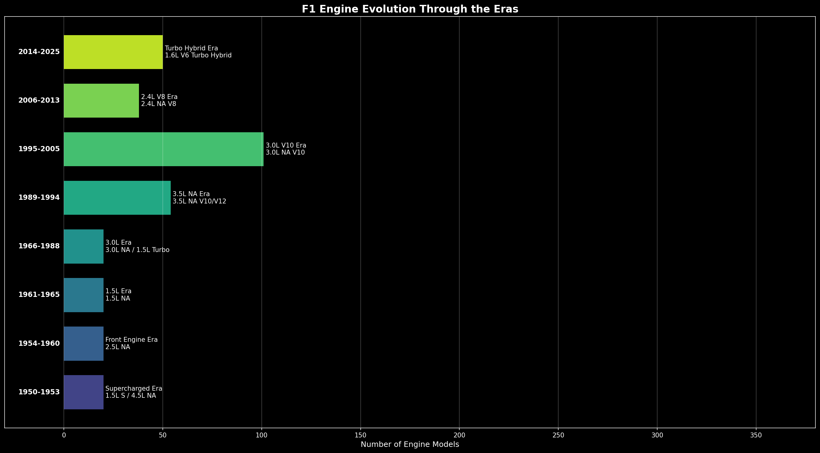
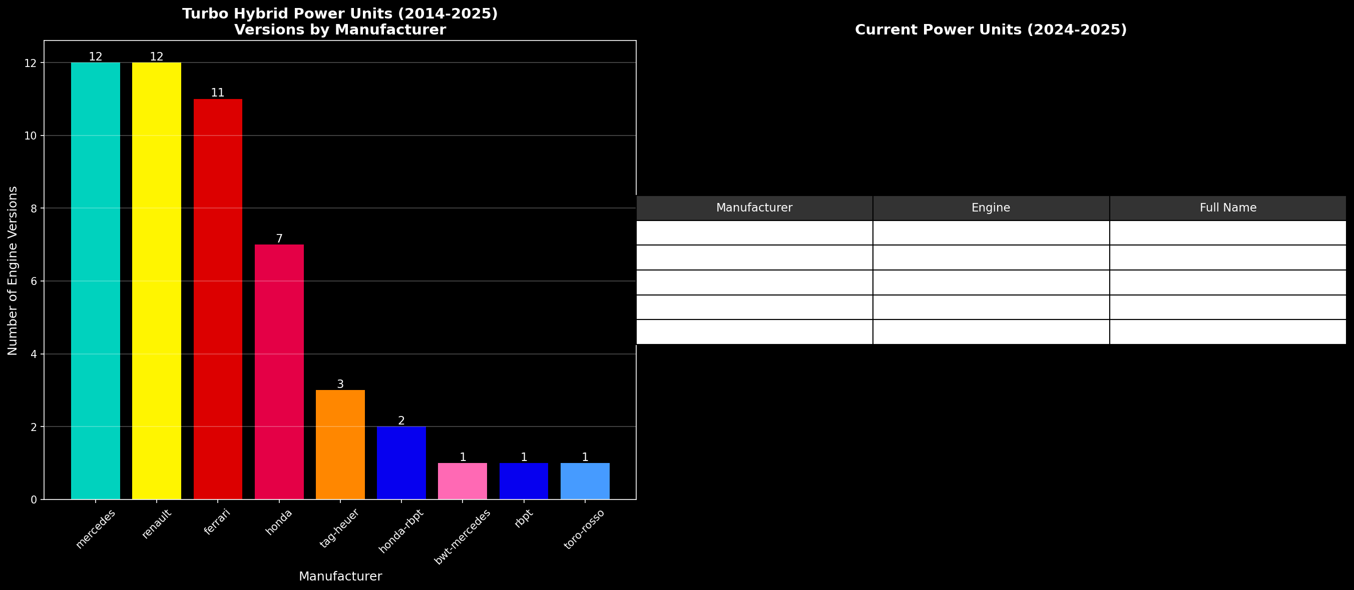
Engine specifications, manufacturer analysis, and hybrid era technology breakdown
The offline twin of the wind tunnel above — the same potential-flow model and the same PERRINN coefficients, rendered at full resolution in Python
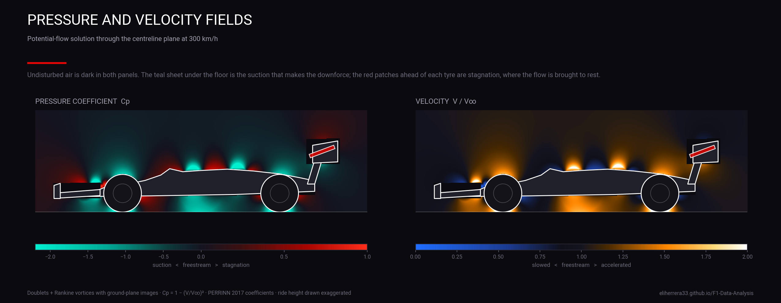
Static pressure and velocity magnitude through the centreline plane, showing the low-pressure region generated under the floor.
Venturi floor behaviour across ride heights, including the stall region.
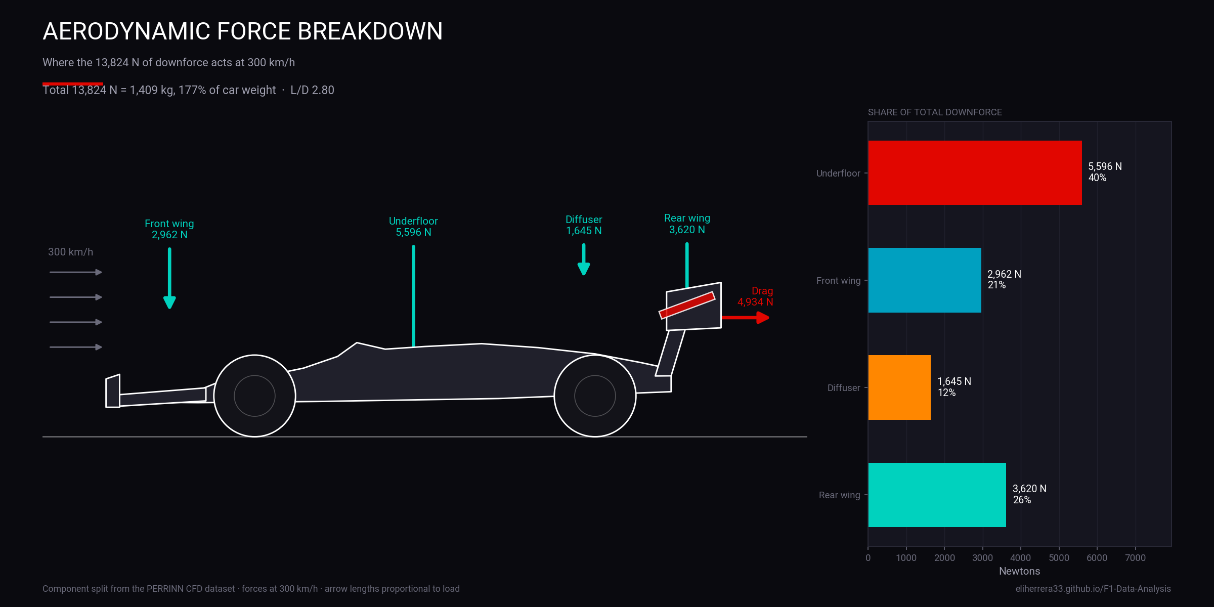
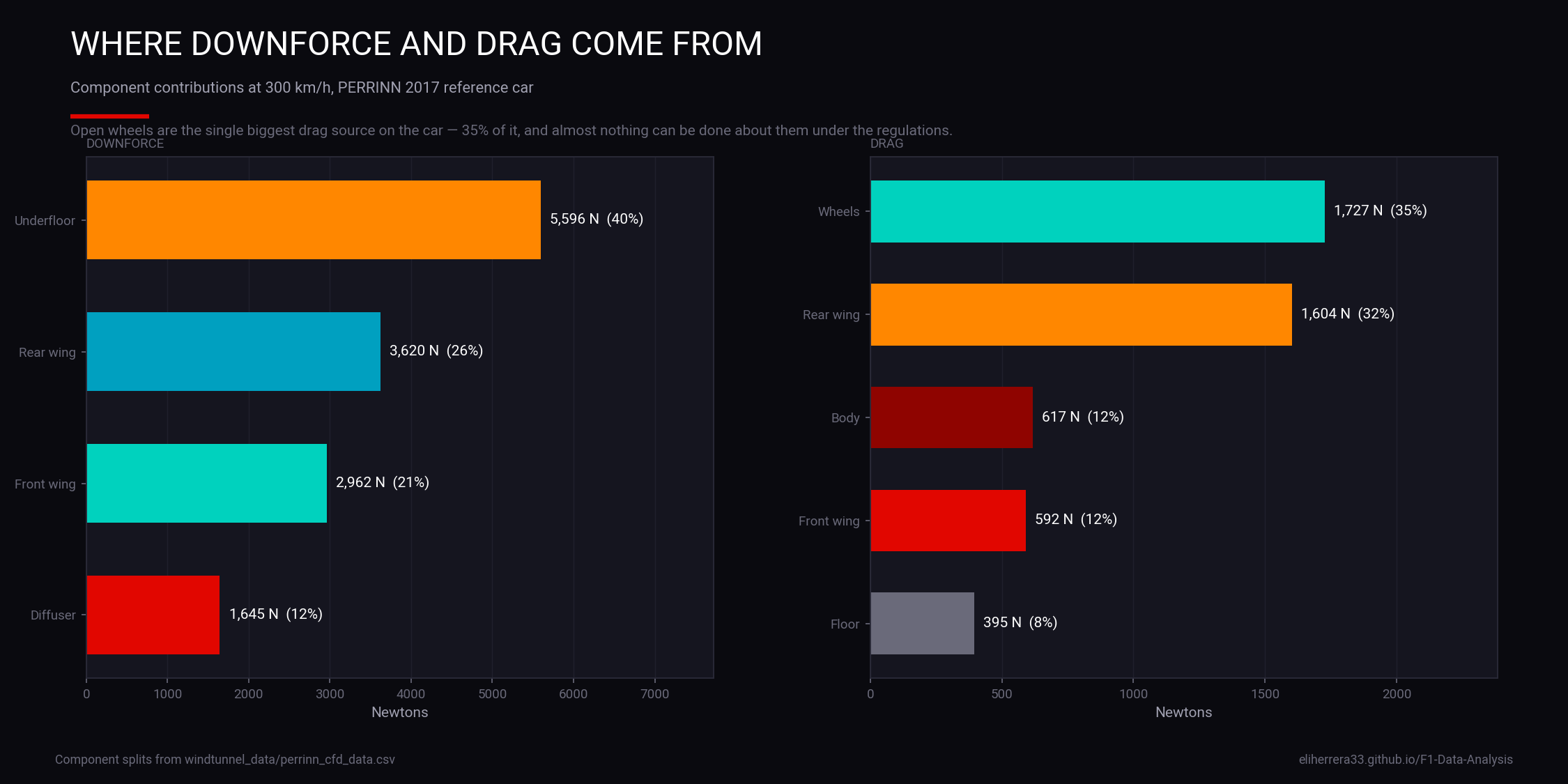
Resolved lift and drag components acting on each aero surface.
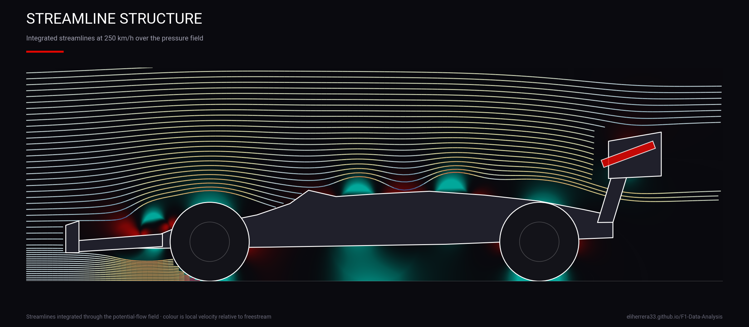
Particles advected through a potential-flow solution — doublets for body thickness, Rankine vortices for circulation, every element mirrored about the ground plane. Colour is Bernoulli pressure: teal where the flow is accelerated and pressure drops, red at the stagnation points ahead of the wheels.
Sweeping the floor from 60 mm down to 15 mm. Downforce climbs as the underfloor works harder, peaks around 24 mm, then collapses as the venturi stalls. That cliff is why the 2022 generation of cars porpoised.
Share of total downforce from floor, front wing, rear wing and bodywork.
Aerodynamic loads sampled from 100 to 350 km/h.
Wake and vortex structure trailing the rear wing endplates.
The two fastest laps of a qualifying session, locked to one clock and under your control. Scrub the lap, watch the gap build, jump to where it was won.
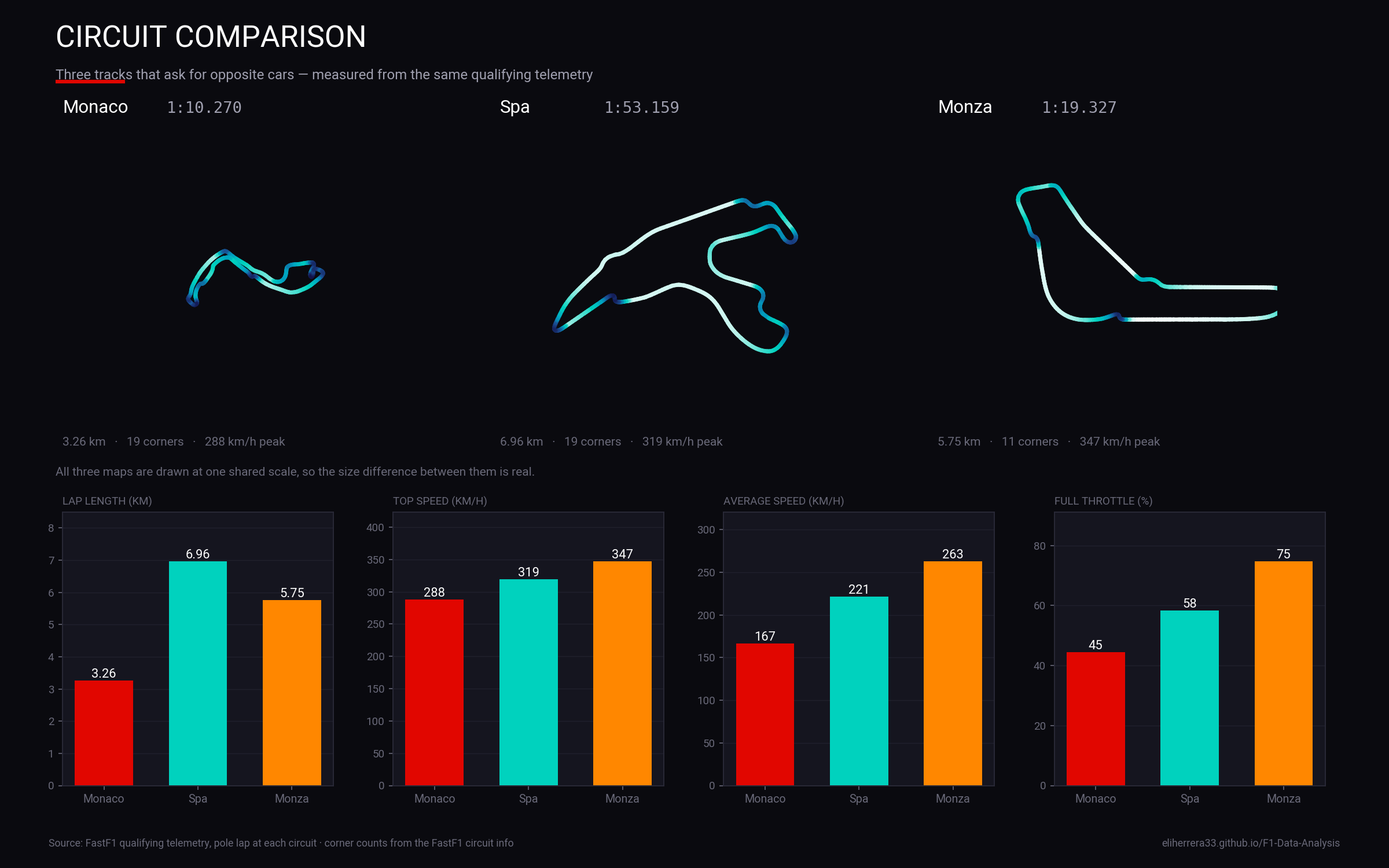
Lap length, corner count and speed profile compared across all three simulated circuits.
Built by Eli Herrera — I build fast, data-heavy web applications. This whole page is the portfolio piece.